Linear Regression
Linear Regression

Regression is probably the first machine learning algorithm you learnt when you first step into the realm of machine learning because of its simplicity and effectiveness it forms the basis for more advanced machine learning algorithms (including neural networks and recommendation algorithms), and is relatively easy to understand.
Regression is a statistical measure that takes a group of random variables and determines a mathematical relationship between them. Expressed differently, regression calculates numerous variables to predict an outcome or score.
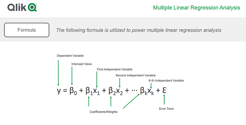
Today we are going to implement linear regression from scratch and plot the line of best fit for our data. To follow along you should have some basic knowledge of python to understand the code and basic understanding of maths. In linear regression we simply apply the formula y=mx + b in 2-dimensional form and the formula becomes more and more complex as we go higher in dimension. So in our formula we have “y” which is the target value which depends on the value of “x” the x-coordinates, “m” which is the slope and “b” the y-intercept.
from statistics import mean
import numpy as np
import matplotlib.pyplot as plt
from matplotlib import style
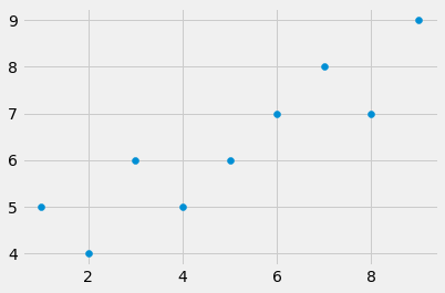
xs= np.array([1, 2 ,3 ,4 ,5 ,6 ,7 , 8, 9], dtype= np.float64)
ys= np.array([5,4,6,5,6,7 ,8, 7 ,9], dtype= np.float64)
First we import the necessary libraries and created x and y numpy arrays. Then we visualise our data using matplotlib library.
plt.scatter(xs,ys) #scatter plot
plt.show()
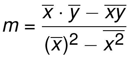
Now we will create functions that will calculate the slope and y-intercept.
def best_slope(xs,ys):
    x_bar = mean(xs)
    y_bar = mean(ys)
    m= (((x_bar * y_bar) - mean(xs*ys)) /
        ((x_bar* x_bar) - mean(xs * xs)))

    return m
def best_intercept(xs , ys):
    y_bar= mean(ys)
    x_bar = mean(xs)
    m=best_slope(xs ,ys)

    b=(y_bar - (m*x_bar))
    return b
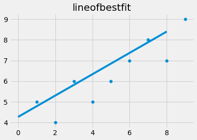
reg_line = [ (m*x) +b for x in xs]
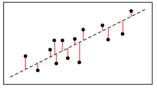
Now we plot the regression line also termed as “line of best fit” with values of m,x and b
plt.scatter(xs, ys)
plt.plot(reg_line)
plt.title(“lineofbestfit”)
plt.show()
But how can we assure that the line predicted by our formula is really the line of best fit. We can do this by calculating the accuracy of the best fit line also known as the R² or the Coefficient of Determination
We calculate this by finding the square of the distance between the data-points and the regression line.
So this is how linear regression really works by finding a line of best find by finding the coefficients of the dependent features to predict the value of output or the target value.
You can check my github link where I provided the i-python notebook for the same which consists of all the codes that I have used here along with it’s explanation. I would like to thank youtube channel “sentdex” for explaining linear regression in such a simple manner you can follow the video by clicking the link below.
My github link: https://github.com/akshayakn13/LinearRegression
Suggestions are always welcomed. Don’t forget to checkout my other articles.
Linear Regression from scratch.

Comments
Post a Comment